Pricing and Hedging Derivative Securities

Binomial Trees

Binomial Trees: Overview

A powerful framework for pricing derivatives using no-arbitrage arguments.

Model stock prices as moving up or down over discrete time steps
Replicate option payoffs using the stock and risk-free asset
Price options by backward induction through the tree
Converges to continuous-time models (Black-Scholes) as steps increase

One-Period Model

One-Period Model: Setup

Stock price $S$ today can take two values at date $t$:

Up state: $S_u$

Down state: $S_d$

Risk-free return: $\mathrm{e}^{rt}$

No-arbitrage condition:

\[S_u/S > \mathrm{e}^{rt} > S_d/S\]

Neither asset dominates the other — no riskless profit possible.

Replicating a Call Option

A European call with strike $K$ pays $C_u = \max(0, S_u - K)$ or $C_d = \max(0, S_d - K)$.

Key insight: We can replicate the option payoff with a portfolio of stock and borrowing.

Define the delta (hedge ratio):

\[\delta = \frac{C_u - C_d}{S_u - S_d}\]

Buy $\delta$ shares, borrow $B = \mathrm{e}^{-rt}(\delta S_u - C_u)$

Replication and No-Arbitrage Pricing

The replicating portfolio matches the option in both states:

Up state: $\delta S_u - B\mathrm{e}^{rt} = C_u$
Down state: $\delta S_d - B\mathrm{e}^{rt} = C_d$

No-arbitrage argument: The option must cost the same as its replicating portfolio:

\[C = \delta S - \mathrm{e}^{-rt}(\delta S_u - C_u)\]

Otherwise, buy the cheap one and sell the expensive one for riskless profit.

Example: Stock Price Tree

Suppose a stock priced at $100 will either go up by 10% or down by 10%.

The simple interest rate is 5% (meaning $\mathrm{e}^{rt}=1.05$). Note $1.10 > 1.05 > 0.90$, so the no-arbitrage condition holds.

Call Option Payoffs

Consider a call option with a strike of $105. It ends with a value of $5 if the stock goes to $110 and $0 if the stock goes to $90.

We want to find its value at the beginning.

Step 1: Compute Delta and Value of $\delta$ Shares

$\delta = (5 - 0)/(110 - 90) = 1/4$. Here is the value of 1/4 share of the stock:

Up state: $0.25 \times 110 = 27.50$
Down state: $0.25 \times 90 = 22.50$

Step 2: Borrowing

Borrow the PV of the down-state portfolio value. At 5% interest, the PV of $22.50 is $21.43.

The debt is the same in both states — it’s risk-free borrowing.

Step 3: Equity = Call Option

The equity in the levered portfolio (shares minus debt) replicates the call:

Up state: $27.50 - 22.50 = 5.00$ = $C_u$
Down state: $22.50 - 22.50 = 0.00$ = $C_d$
Call value = cost of $\delta$ shares $-$ amount borrowed $= 25.00 - 21.43 = 3.57$

State Prices

Define state prices — the cost today of $1 in a single state:

\[\pi_u = \frac{S - \mathrm{e}^{-rt}S_d}{S_u - S_d}, \quad \pi_d = \frac{\mathrm{e}^{-rt}S_u - S}{S_u - S_d}\]

Every asset can be valued as a portfolio of state payoffs:

Call: $C = \pi_u C_u + \pi_d C_d$
Stock: $S = \pi_u S_u + \pi_d S_d$
Risk-free: $1 = \pi_u \mathrm{e}^{rt} + \pi_d \mathrm{e}^{rt}$

No-arbitrage implies $\pi_u > 0$ and $\pi_d > 0$.

Risk-Neutral Pricing

Transform state prices into risk-neutral probabilities: $p_u = \mathrm{e}^{rt}\pi_u$, $p_d = \mathrm{e}^{rt}\pi_d$

$p_u + p_d = 1$ and both positive — mathematical probabilities
Not anyone’s actual beliefs — artificial probabilities

Pricing formulas:

\[C = \mathrm{e}^{-rt}\big[p_u C_u + p_d C_d\big]\] \[S = \mathrm{e}^{-rt}\big[p_u S_u + p_d S_d\big]\]

Value = discounted expected payoff using risk-neutral probabilities.

Risk-Neutral Probabilities: Example

Return to our example. If there were no risk premium, the stock price would be the discounted expected value:

\[\$100 = \frac{p \times \$110 + (1-p) \times \$90}{1.05}\]

Solving for $p$:

\[p = \frac{r_f - r_d}{r_u - r_d} = \frac{0.05 - (-0.10)}{0.10 - (-0.10)} = \frac{0.15}{0.20} = 0.75\]

Call value:

\[C = \frac{0.75 \times \$5 + 0.25 \times \$0}{1.05} = \$3.57\]

Same answer as the delta hedge — because it’s just algebra!

Computing Risk-Neutral Probabilities

Directly from asset returns:

\[p_u = \frac{\mathrm{e}^{rt} - S_d/S}{S_u/S - S_d/S}, \quad p_d = 1 - p_u\]

Numerator: risk-free return minus down return
Denominator: up return minus down return
Same formula extends to multiperiod trees (replacing $t$ with $\Delta t$)

Why Does Risk-Neutral Pricing Work?

The delta hedge argument didn’t depend on risk preferences
So we can act as if investors don’t require risk premia
The risk-neutral probabilities are not anyone’s actual beliefs
They are simply a convenient computational tool derived from no-arbitrage

Two-Period Model

Backward Induction

Work backwards from maturity to find today’s value:

Step 1 — Terminal payoffs:

$C_{uu} = \max(0, u^2S - K)$, $\;C_{ud} = \max(0, S - K)$, $\;C_{dd} = \max(0, d^2S - K)$

Step 2 — Intermediate nodes:

$C_u = \mathrm{e}^{-r\Delta t}[p \cdot C_{uu} + (1-p) \cdot C_{ud}]$
$C_d = \mathrm{e}^{-r\Delta t}[p \cdot C_{ud} + (1-p) \cdot C_{dd}]$

Step 3 — Today’s value:

$C_0 = \mathrm{e}^{-r\Delta t}[p \cdot C_u + (1-p) \cdot C_d]$

Two-Period Stock Tree

Suppose a $100 stock goes up by 5% or down by $(1/1.05 - 1) = -4.76\%$ in each of two periods.

The tree recombines: up then down = down then up = $100. The interest rate is 3% per period.

Two-Period Call (K = $105)

A call with strike $105 expires at the end of the 2nd period. Terminal payoffs:

We need to work backwards to fill in the values at earlier nodes.

Backward Induction: Delta Hedging

At each intermediate node, repeat the one-period analysis:

At the up node ($S = 105$): use payoffs $C_{uu} = 5.25$ and $C_{ud} = 0$ to find $C_u$

At the down node ($S = 95.24$): use payoffs $C_{ud} = 0$ and $C_{dd} = 0$ to find $C_d$

At the initial node ($S = 100$): use $C_u$ and $C_d$ to find $C_0$

This recursive procedure is backward induction.

Risk-Neutral Probability

The risk-neutral probability of “up” each period is:

\[p = \frac{r_f - r_d}{r_u - r_d} = \frac{0.03 - (-0.0476)}{0.05 - (-0.0476)} = 0.795\]

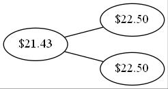
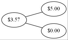
Discounting the expected call values at the risk-free rate yields:

Another Example: Call with K = $95

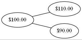
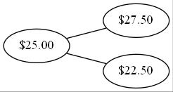
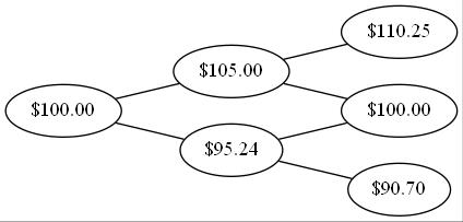
Stock tree:

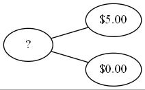
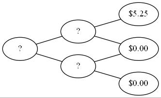
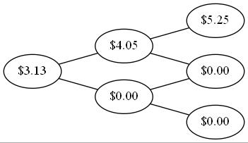
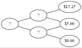
Call with strike $95:

Apply the same backward induction to fill in the intermediate and initial values.

Two-Period Example in Code

S = 100
K = 95
u = 0.05            # up return per period
r = 0.03            # interest rate per period
n = 2               # number of periods
d = 1/(1+u) - 1     # down return per period
p = (r-d) / (u-d)   # risk-neutral prob

# Terminal stock prices and call payoffs
x = [S*(1+u)**(n-2*i) for i in range(n+1)]
v = np.maximum(0, np.array(x)-K)

# Backward induction
while len(v) > 1:
    v = (p*v[:-1] + (1-p)*v[1:]) / (1+r)

print(f"Risk-neutral prob p = {p:.4f}")
print(f"Call value (K={K}): ${v[0]:.2f}")

Risk-neutral prob p = 0.7951
Call value (K=95): $10.62

American Options: Early Exercise

At each intermediate node, compare continuation vs. immediate exercise:

\[V = \max\!\big(\text{continuation value},\; \text{exercise value}\big)\]

Continuation: $\mathrm{e}^{-r\Delta t}[p \cdot V_u + (1-p) \cdot V_d]$
Exercise (call): $\max(0, S - K)$
Exercise (put): $\max(0, K - S)$

Backward induction automatically finds the optimal exercise strategy.

N-Period Model

N-Period Extension

With $N$ periods, after $n$ steps there are $n+1$ nodes:

\[S_j = u^j d^{n-j} S = u^{2j-n}S, \quad j = 0, 1, \ldots, n\]

Tree recombines because $ud = 1$
Total nodes = $\frac{(N+1)(N+2)}{2}$ (much less than $2^N$ paths)
Backward induction is efficient: work one time step at a time

Interactive N-Period Trees

Figure 1: Experiment with N-period binomial trees: adjust interest rates, up/down factors, number of periods, and compare European vs. American option pricing.

Vectorized Implementation

import numpy as np

def binomial_american(S0, K, r, sigma, T, N, option_type='put'):
    dt = T / N
    u = np.exp(sigma * np.sqrt(dt))
    d = 1 / u
    p = (np.exp(r * dt) - d) / (u - d)
    disc = np.exp(-r * dt)

    # Terminal payoffs
    j = np.arange(N + 1)
    S = S0 * u**j * d**(N - j)
    V = np.maximum(K - S, 0) if option_type == 'put' else np.maximum(S - K, 0)

    # Backward induction
    for i in range(N - 1, -1, -1):
        j = np.arange(i + 1)
        S = S0 * u**j * d**(i - j)
        V = disc * (p * V[1:i+2] + (1-p) * V[0:i+1])
        exercise = np.maximum(K - S, 0) if option_type == 'put' else np.maximum(S - K, 0)
        V = np.maximum(V, exercise)

    return V[0]

print(f"American put:  {binomial_american(100, 105, 0.05, 0.2, 1, 100, 'put'):.4f}")
print(f"American call: {binomial_american(100, 105, 0.05, 0.2, 1, 100, 'call'):.4f}")

American put:  8.7476
American call: 8.0262

How the Algorithm Works

Vectorization: NumPy arrays compute all nodes at each time step simultaneously
Memory efficiency: Only store option values for the current time step
Backward induction logic:
- Start with payoffs at maturity
- At each prior step: discounted expected value of next period
- Compare to immediate exercise (American feature)
- Take the maximum

Parameter Calibration and Convergence

Parameter Calibration: CRR

Cox-Ross-Rubinstein parameters match the continuous-time limit:

\[u = \mathrm{e}^{\sigma\sqrt{\Delta t}}, \quad d = \frac{1}{u}, \quad p = \frac{\mathrm{e}^{(r-q)\Delta t} - d}{u - d}\]

$\sigma$ = volatility of the underlying
$q$ = dividend yield
Tree recombines: $ud = 1$
Converges to geometric Brownian motion as $\Delta t \to 0$

Convergence to Black-Scholes

Figure 2: Binomial model (blue dots) converges to the Black-Scholes limit (red line) as the number of time steps increases. Deviations are the same for calls and puts, reflecting put-call parity.

Summary: Key Takeaways

Replication: Option payoffs can be replicated with stock + borrowing
No-arbitrage pricing: Option value = cost of replicating portfolio
Risk-neutral probabilities: Value = discounted expected payoff under artificial probabilities
Backward induction: Work from maturity to today, comparing continuation vs. exercise at each node
CRR calibration: $u = \mathrm{e}^{\sigma\sqrt{\Delta t}}$, $d = 1/u$ ensures convergence to Black-Scholes
American options: Backward induction automatically finds optimal exercise strategy